Getting Started
Input Expressions
Options
Input
Caladis makes it easy to perform calculations involving probability distributions. To perform a calculation, enter a mathematical expression in the input box on the home page. Mathematical expressions can include numbers, operators, functions and constants (see INPUT EXPRESSIONS for more details). A simple expression might take the form:
1 + 2
This expression does not include any probability distributions so will have a single solution (in this case 3). To make our expression probabilistic we must add a probability distribution variable. These are defined using the hash symbol, #, and can include upper-case letters, lower-case letters and numbers 0-9. Adding to our previous example, we define a distribution variable called "myDistribution":
1 + 2 + #myDistribution
As we type the variable's name, Caladis produces a popup enabling us to define what type of probability distribution our variable is:
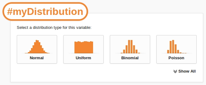
The popup lists all of the available probability distributions in Caladis. To select a distribution type simply click on its icon.
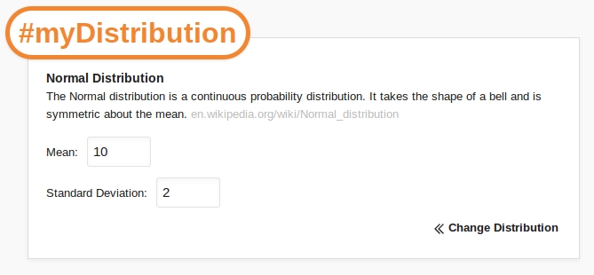
When a distribution is selected (in this case the Normal distribution), the content of the popup changes so that the distribution parameters can be entered. In the case of the Normal distribution we must define the Mean and Standard Deviation. Once these details have been entered we click Calculate.
Compute
The compute page shows the results from Caladis' calculations. At the top of the page is the input expression.

Distribution variables are highlighted in orange and a distribution's parameters can be seen by hovering the cursor over its name.
Caladis uses Monte Carlo sampling to generate its results. The input expression is calculated repeatedly, each time selecting a random number from each of the input probability distributions. The results of these calculations are displayed as a histogram on the Compute page:
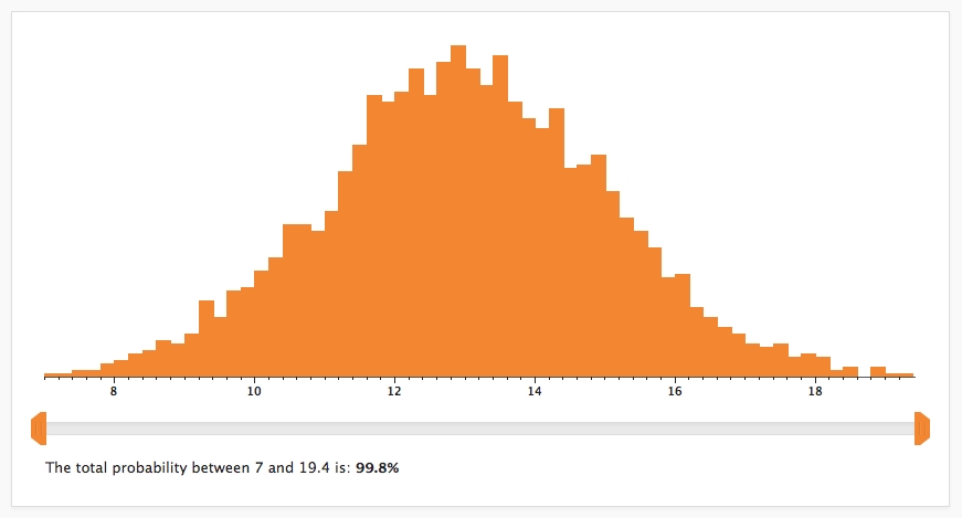
Each bar of the histogram shows the percentage of data points that fell between the upper and lower bounds of that bar. The slider-bar beneath the histogram can be used to show the percentage of data points that lie between any two points. These points can be changed by moving the two orange tabs at either end of the slider-bar.
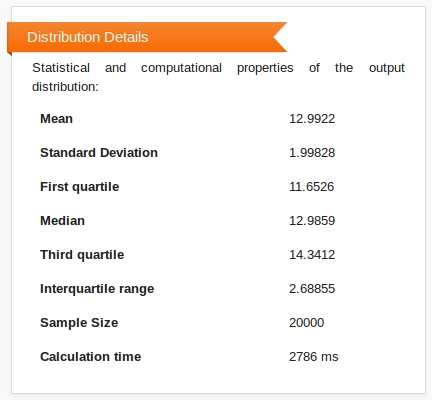
Summary statistics of the distribution, including mean, median, standard deviation and interquartile range, are presented in a box below the histogram.
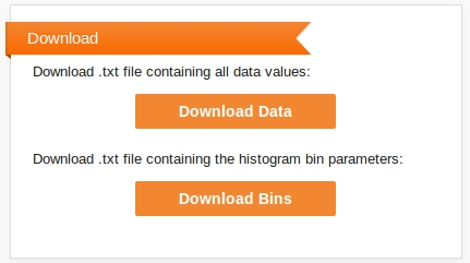
A second box allows you to download the raw data that was used in producing the histogram (the set of samples from the output distribution), and the data grouped into the histogram bins.
Operators
The following operators can be used in input expressions.
| Operator | Description |
|---|---|
| + | Addition |
| - | Subtraction |
| * | Multiplication |
| / | Division |
| ^ | Exponentiation, i.e. "to the power of" |
If negative numbers or functions are to be included as exponents (following the ^ operator), please enclose them in brackets:
10^(-3) * 2^(exp(#n))
Functions
The following functions can be used in input expressions.
| Function | Description |
|---|---|
| abs() | Returns the absolute value of a number. |
| acos() | Returns the arccosine of a number. |
| acosh() | Returns the inverse hyperbolic cosine of a number. |
| asin() | Returns the arcsine of a number. |
| asinh() | Returns the inverse hyperbolic sine of a number. |
| atan() | Returns the arctangent of a number as a numeric value between -π/2 and π/2 radians. |
| atanh() | Returns the inverse hyperbolic tangent of a number. |
| ceil() | Returns the value of a number rounded upwards to the nearest integer. |
| cos() | Returns the cosine of a number. |
| cosh() | Returns the hyperbolic cosine of a number. |
| exp() | Returns the value of e^x. |
| floor() | Returns the value of a number rounded downwards to the nearest integer. |
| log() | Returns the natural logarithm (base e) of a number. |
| round() | Rounds a number to the nearest integer. |
| sin() | Returns the sine of a number. |
| sinh() | Returns the hyperbolic sine of a number. |
| tan() | Returns the tangent of an angle. |
| tanh() | Returns the hyperbolic tangent of an angle. |
Constants
Entering
pi
in the input expression automatically includes π, approximately equal to 3.14159.
To enter numerical constants in scientific notation, use inputs of the form
1.5 * 10^5
If negative numbers or functions are to be used as exponents, enclose them in brackets:
10^(-3) * 2^(exp(#n))
Standard Deviation Analysis
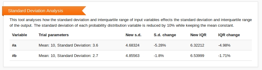
Standard Deviation Analysis investigates how the standard deviation of the input variables affect the standard deviation and interquartile range of the output. For each distribution defined, the standard deviation is reduced by 10% and the effect of this change on the output distribution is calculated. The results of this analysis are shown beneath the histogram on the Compute page.
By default, Standard Deviation Analysis is turned off.
Sample Size
The Sample Size option determines how many calculations will be used to generate the results. Increasing the Sample Size improves the accuracy of the results but takes longer to compute.
By default, the sample size is 20,000.
Use Bionumbers
The Bionumbers website is a repository of useful numbers in biology, encompassing a wide range of topics from rates of metabolic chemical reactions to the number of bacteria in a termite's gut. These numbers have been recorded from experiments and are usually stored as a value with some associated uncertainty (perhaps due to experimental errors, or natural variability). Caladis can help perform biological calculations by automatically including your choice of Bionumbers in your calculations.
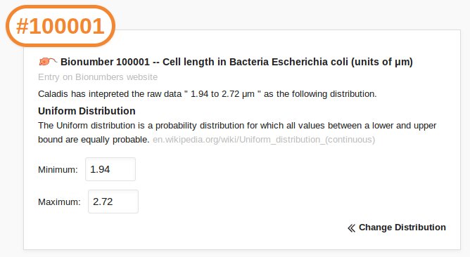
Caladis automatically recognises Bionumber references preceded by hashes and include the corresponding distribution in your calculations: for example, entering "#100001" references the Bionumber corresponding to the length of an E. coli bacterium. Caladis interprets the raw data from the Bionumbers database as probability distributions by examining the format of the number and its associated range.
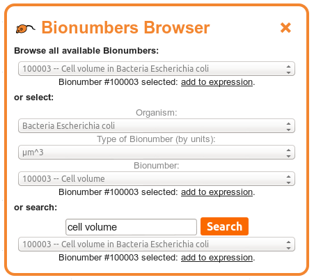
The "Bionumbers Browser" allows you to browse the full list of Bionumber references, to select Bionumbers using a three-tiered process by organism and type of Bionumber, or to search the Bionumbers database.
To select a Bionumber using the three-tiered process, first select the organism that you are interested in obtaining a Bionumber for from the top menu. The next menu will now display all types of Bionumber available for that organism, listed by the associated units of the Bionumbers: for example, cellular volumes may have associated units of μm3. Select the type of Bionumber you are interested in from this menu. The bottom menu will now contain all Bionumbers of that unit in that organism, from which you may select the quantity of interest.
To search for a Bionumber, enter your search term(s) into the search bar available. Caladis will search the descriptions of each Bionumber for your terms. If you enter more than one search term, separated by spaces, Caladis will first attempt to find description that match all of the terms you enter. If no Bionumbers exist matching all your search search, Caladis will next attempt to find Bionumber matching at least one of your search terms. If any Bionumbers match these searches, they will be presented in the menu below the search bar.
After selecting a Bionumber from any of the above three approaches, a link will appear below your choice allowing you to insert that Bionumber directly into Caladis' expression bar.
Some Bionumbers appear in the database without an estimate of their associated uncertainty. Caladis will automatically assign a large uncertainty (a standard deviation of half the Bionumber's value) to these numbers, and provide a link to the website entry so you can check the appropriate values.
An option in Caladis' option set enables you to influence how Caladis interprets some Bionumbers. Some values are present in the database with errors in the form "x +/- y", and some as "a to b" or "a-b" (as well as other variations). By default, Caladis interprets these types of value respectively as normally distributed with mean x and standard deviation y and uniformly distributed between a and b. The menu option allows you to interpret data of these type as log-normally distributed, which is more appropriate in some biological contexts (for example, when the Bionumber is known to be non-negative). Respectively, the log-normal distributions used have mean x and standard deviation y, or a and b as the +/- one standard deviation points in the distribution.
By default, Bionumbers with "x +/- y" range information are intepreted as normal, and those with "x to y" range information are interpreted as uniform.
Binning Method
The Binning Method option determines how the number of bins in the histogram be calculated. Rather than inputting the number of bins directly, Caladis lets users choose from three methods for deriving the optimal number of bins:
Freedman-Diaconis (default)
The Freedman-Diaconis rule is based on the interquartile range. It gives the width of each bin as:
w = 2 * IQR * ( n ^ (-1/3) )
where IQR is the interquartile range and n is the number of data points.
Scott
Scott's rule is optimal for random samples of normally distributed data, in the sense that it minimises the integrated mean squared error of the density estimate. It gives the width of each bin as:
w = 3.5 * σ * ( n ^ (-1/3) )
where σ is the standard deviation and n is the number of data points.
Sturges
Sturges' formula is derived from a binomial distribution and implicitly assumes an approximately normal distribution. It gives the number of bins as:
k = ceil( log2n + 1 )
where n is the number of data points.
Angle Unit
The Angle Unit option determines the unit used in trigonometric functions.
By default, the angle unit is radians.